Composites#

Plotting individual bands is good but we usually want to make some composite images to visualize information from multiple bands at once. For that, we have to create composites. We provide the xlandsat.composite function to make this process easier.

As an example, let’s load two example scenes from the Brumadinho tailings dam disaster:

import xlandsat as xls
import matplotlib.pyplot as plt

path_before = xls.datasets.fetch_brumadinho_before()
path_after = xls.datasets.fetch_brumadinho_after()

before = xls.load_scene(path_before)
after = xls.load_scene(path_after)

Creating composites#

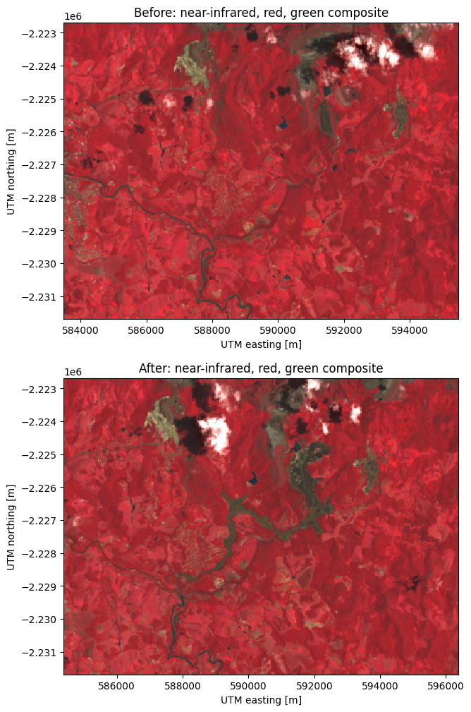
Let’s make both RGB (true color) and CIR (color infrared) composites for both of our scenes:

The composites have a similar layout as the bands but with an extra "channel" dimension corresponding to red, green, blue, and alpha/transparency. The values are scaled to the [0, 255] range and the composite is an array of unsigned 8-bit integers.

Transparency

If any of the bands used for the composite have NaNs, those pixels will have their transparency set to the maximum value of 255. If there are no NaNs in any band, then the composite will only have 3 channels (red, green, blue).

Now do the same for the after scene:

Plotting composites#

Composites can be plotted using xarray.DataArray.plot.imshow (using plot won’t work and will display histograms instead). Let’s make the before and after figures again for each of the composites we generated.

fig, (ax1, ax2) = plt.subplots(2, 1, figsize=(10, 12))

# Plot the composites
before.rgb.plot.imshow(ax=ax1)
after.rgb.plot.imshow(ax=ax2)

# The "long_name" of the composite is the band combination
ax1.set_title(f"Before: {before.rgb.attrs['long_name']}")
ax2.set_title(f"After: {after.rgb.attrs['long_name']}")

ax1.set_aspect("equal")
ax2.set_aspect("equal")

plt.show()

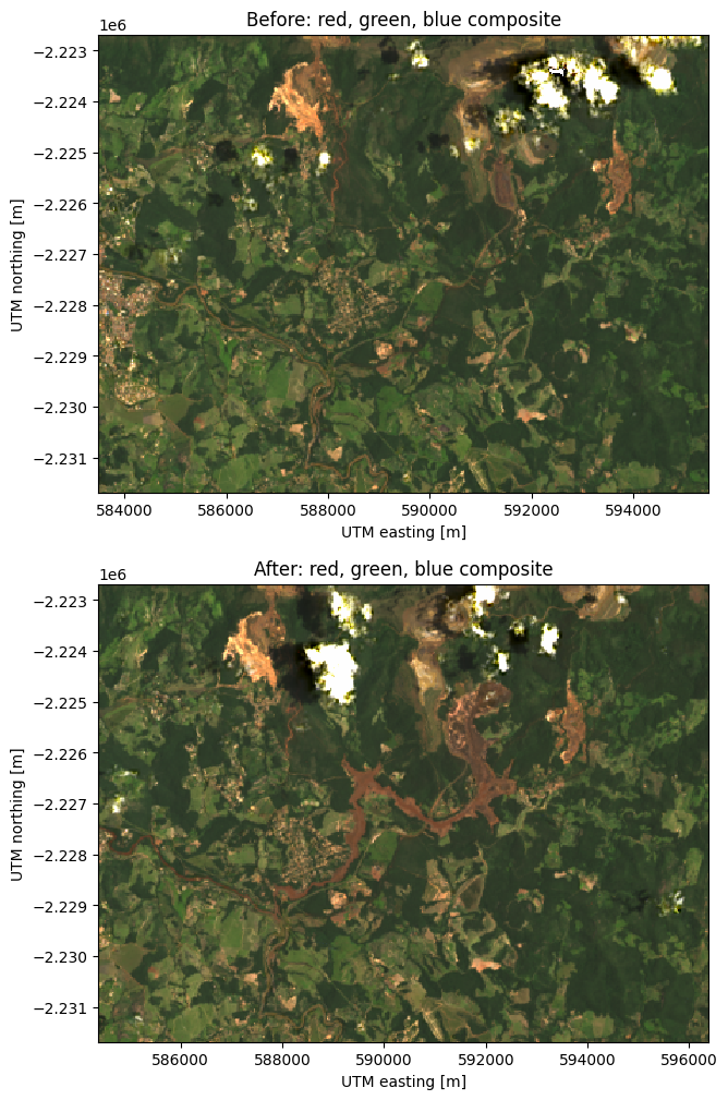
And now the CIR composites:

fig, (ax1, ax2) = plt.subplots(2, 1, figsize=(10, 12))

before.cir.plot.imshow(ax=ax1)
after.cir.plot.imshow(ax=ax2)

ax1.set_title(f"Before: {before.cir.attrs['long_name']}")
ax2.set_title(f"After: {after.cir.attrs['long_name']}")

ax1.set_aspect("equal")
ax2.set_aspect("equal")

plt.show()

xlandsat v0.3.0

Composites

Contents

Composites#

Creating composites#

Plotting composites#