Overview
Contents
Overview#
The library#
All functionality in xlandsat is available from the base namespace of the
xlandsat package. This means that you can access all of them with a
single import:
# xlandsat is usually imported as xls
import xlandsat as xls
Download a sample scene#
As an example, lets download a tar archive of a Landsat 8 scene of the Brumadinho tailings dam disaster that happened in 2019 in Brazil. The archive is available on figshare at https://doi.org/10.6084/m9.figshare.21665630 and includes scenes from before and after the disaster as both the full scene and a cropped version.
We’ll use the functions in xlandsat.datasets to download the scenes from
before and after the disaster to our computer. To save space and bandwidth,
these are cropped versions of the full Landsat scenes.
path_before = xls.datasets.fetch_brumadinho_before()
path_after = xls.datasets.fetch_brumadinho_after()
print(path_before)
print(path_after)
/home/runner/.cache/pooch/LC08_L2SP_218074_20190114_20200829_02_T1-cropped.tar.gz
/home/runner/.cache/pooch/LC08_L2SP_218074_20190130_20200829_02_T1-cropped.tar.gz
Tip
Running the code above will only download the data once. We use Pooch to handle the downloads and it’s smart
enough to check if the file already exists on your computer. See
pooch.retrieve for more information.
See also
If you want to use the full scenes instead of the cropped version,
use pooch.retrieve to fetch them from the figshare archive
https://doi.org/10.6084/m9.figshare.21665630.
Load the scenes#
Now that we have paths to the tar archives of the scenes, we can use
xlandsat.load_scene to read the bands and metadata directly from the
archives (without unpacking):
before = xls.load_scene(path_before)
before
<xarray.Dataset>
Dimensions:   (easting: 400, northing: 300)
Coordinates:
  * easting   (easting) float64 5.835e+05 5.835e+05 ... 5.954e+05 5.955e+05
  * northing  (northing) float64 -2.232e+06 -2.232e+06 ... -2.223e+06 -2.223e+06
Data variables:
    blue      (northing, easting) float16 0.07288 0.07373 ... 0.06506 0.06653
    green     (northing, easting) float16 0.09851 0.099 ... 0.0835 0.08716
    red       (northing, easting) float16 0.1035 0.1041 ... 0.07959 0.08423
    nir       (northing, easting) float16 0.2803 0.2749 0.3203 ... 0.2118 0.2267
    swir1     (northing, easting) float16 0.2467 0.2474 0.2147 ... 0.172 0.1769
    swir2     (northing, easting) float16 0.1571 0.1571 0.1281 ... 0.1171 0.1206
Attributes: (12/19)
    Conventions:                CF-1.8
    title:                      Landsat 8 scene from 2019-01-14 (path/row=218...
    digital_object_identifier:  https://doi.org/10.5066/P9OGBGM6
    origin:                     Image courtesy of the U.S. Geological Survey
    landsat_product_id:         LC08_L2SP_218074_20190114_20200829_02_T1
    processing_level:           L2SP
    ...                         ...
    ellipsoid:                  WGS84
    date_acquired:              2019-01-14
    scene_center_time:          12:57:13.1804960Z
    wrs_path:                   218
    wrs_row:                    74
mtl_file: GROUP = LANDSAT_METADATA_FILE\n GROUP = PROD...- easting: 400
- northing: 300
- easting(easting)float645.835e+05 5.835e+05 ... 5.955e+05
- long_name :
- UTM easting
- standard_name :
- projection_x_coordinate
- units :
- m
array([583500., 583530., 583560., ..., 595410., 595440., 595470.])
- northing(northing)float64-2.232e+06 ... -2.223e+06
- long_name :
- UTM northing
- standard_name :
- projection_y_coordinate
- units :
- m
array([-2231670., -2231640., -2231610., ..., -2222760., -2222730., -2222700.])
- blue(northing, easting)float160.07288 0.07373 ... 0.06506 0.06653
- long_name :
- blue
- units :
- reflectance
- number :
- 2
- filename :
- LC08_L2SP_218074_20190114_20200829_02_T1_SR_B2.TIF
- scaling_mult :
- 2e-05
- scaling_add :
- -0.1
array([[0.0729 , 0.0737 , 0.06934, ..., 0.06396, 0.06165, 0.06604], [0.074 , 0.07263, 0.0768 , ..., 0.06128, 0.06042, 0.07117], [0.0748 , 0.0719 , 0.07556, ..., 0.05957, 0.05676, 0.06177], ..., [0.06494, 0.06238, 0.063 , ..., 0.0652 , 0.0663 , 0.0657 ], [0.067 , 0.0647 , 0.06238, ..., 0.0647 , 0.06506, 0.0663 ], [0.067 , 0.0665 , 0.06396, ..., 0.067 , 0.06506, 0.0665 ]], dtype=float16) - green(northing, easting)float160.09851 0.099 ... 0.0835 0.08716
- long_name :
- green
- units :
- reflectance
- number :
- 3
- filename :
- LC08_L2SP_218074_20190114_20200829_02_T1_SR_B3.TIF
- scaling_mult :
- 2e-05
- scaling_add :
- -0.1
array([[0.0985 , 0.099 , 0.09326, ..., 0.0919 , 0.08264, 0.0841 ], [0.1024 , 0.1 , 0.1045 , ..., 0.08496, 0.0891 , 0.1034 ], [0.103 , 0.1 , 0.10266, ..., 0.084 , 0.0764 , 0.07495], ..., [0.08496, 0.07935, 0.0807 , ..., 0.0842 , 0.0842 , 0.0825 ], [0.0875 , 0.083 , 0.0774 , ..., 0.08374, 0.08264, 0.0846 ], [0.0873 , 0.08704, 0.0814 , ..., 0.0852 , 0.0835 , 0.08716]], dtype=float16) - red(northing, easting)float160.1035 0.1041 ... 0.07959 0.08423
- long_name :
- red
- units :
- reflectance
- number :
- 4
- filename :
- LC08_L2SP_218074_20190114_20200829_02_T1_SR_B4.TIF
- scaling_mult :
- 2e-05
- scaling_add :
- -0.1
array([[0.1035 , 0.1041 , 0.08704, ..., 0.0834 , 0.074 , 0.0796 ], [0.109 , 0.1029 , 0.1073 , ..., 0.06934, 0.07825, 0.1046 ], [0.1078 , 0.103 , 0.10657, ..., 0.0707 , 0.0657 , 0.0668 ], ..., [0.07886, 0.07263, 0.07336, ..., 0.0764 , 0.0803 , 0.0779 ], [0.0819 , 0.0785 , 0.0714 , ..., 0.07544, 0.0773 , 0.0812 ], [0.08093, 0.08167, 0.07434, ..., 0.0801 , 0.0796 , 0.0842 ]], dtype=float16) - nir(northing, easting)float160.2803 0.2749 ... 0.2118 0.2267
- long_name :
- near-infrared
- units :
- reflectance
- number :
- 5
- filename :
- LC08_L2SP_218074_20190114_20200829_02_T1_SR_B5.TIF
- scaling_mult :
- 2e-05
- scaling_add :
- -0.1
array([[0.2803, 0.275 , 0.3203, ..., 0.2832, 0.2905, 0.2773], [0.2837, 0.2915, 0.3047, ..., 0.3032, 0.2827, 0.2847], [0.3018, 0.3042, 0.2983, ..., 0.3213, 0.2598, 0.2573], ..., [0.2394, 0.2291, 0.2191, ..., 0.2465, 0.2301, 0.2184], [0.2382, 0.2177, 0.1993, ..., 0.2423, 0.2177, 0.2169], [0.2443, 0.2301, 0.2191, ..., 0.2274, 0.2118, 0.2267]], dtype=float16) - swir1(northing, easting)float160.2467 0.2474 ... 0.172 0.1769
- long_name :
- short-wave infrared 1
- units :
- reflectance
- number :
- 6
- filename :
- LC08_L2SP_218074_20190114_20200829_02_T1_SR_B6.TIF
- scaling_mult :
- 2e-05
- scaling_add :
- -0.1
array([[0.2467, 0.2474, 0.2147, ..., 0.1874, 0.1725, 0.1915], [0.2559, 0.2457, 0.2457, ..., 0.1827, 0.1815, 0.2103], [0.254 , 0.2401, 0.2443, ..., 0.1681, 0.1539, 0.16 ], ..., [0.1937, 0.1664, 0.1654, ..., 0.1766, 0.1766, 0.1708], [0.194 , 0.1859, 0.1525, ..., 0.1727, 0.1715, 0.1759], [0.1874, 0.1896, 0.1632, ..., 0.1766, 0.172 , 0.1769]], dtype=float16) - swir2(northing, easting)float160.1571 0.1571 ... 0.1171 0.1206
- long_name :
- short-wave infrared 2
- units :
- reflectance
- number :
- 7
- filename :
- LC08_L2SP_218074_20190114_20200829_02_T1_SR_B7.TIF
- scaling_mult :
- 2e-05
- scaling_add :
- -0.1
array([[0.1571 , 0.1571 , 0.128  , ..., 0.1245 , 0.10156, 0.1112 ],
       [0.163  , 0.1552 , 0.1576 , ..., 0.1067 , 0.10864, 0.1364 ],
       [0.161  , 0.1503 , 0.1534 , ..., 0.10046, 0.0897 , 0.0929 ],
       ...,
       [0.1216 , 0.1045 , 0.10547, ..., 0.11475, 0.11755, 0.11523],
       [0.125  , 0.1205 , 0.1    , ..., 0.1122 , 0.11475, 0.1199 ],
       [0.11926, 0.1206 , 0.10474, ..., 0.1194 , 0.11707, 0.1206 ]],
      dtype=float16)
- eastingPandasIndex
PandasIndex(Float64Index([583500.0, 583530.0, 583560.0, 583590.0, 583620.0, 583650.0, 583680.0, 583710.0, 583740.0, 583770.0, ... 595200.0, 595230.0, 595260.0, 595290.0, 595320.0, 595350.0, 595380.0, 595410.0, 595440.0, 595470.0], dtype='float64', name='easting', length=400)) - northingPandasIndex
PandasIndex(Float64Index([-2231670.0, -2231640.0, -2231610.0, -2231580.0, -2231550.0,
              -2231520.0, -2231490.0, -2231460.0, -2231430.0, -2231400.0,
              ...
              -2222970.0, -2222940.0, -2222910.0, -2222880.0, -2222850.0,
              -2222820.0, -2222790.0, -2222760.0, -2222730.0, -2222700.0],
             dtype='float64', name='northing', length=300))
- Conventions :
- CF-1.8
- title :
- Landsat 8 scene from 2019-01-14 (path/row=218/74)
- digital_object_identifier :
- https://doi.org/10.5066/P9OGBGM6
- origin :
- Image courtesy of the U.S. Geological Survey
- landsat_product_id :
- LC08_L2SP_218074_20190114_20200829_02_T1
- processing_level :
- L2SP
- collection_number :
- 02
- collection_category :
- T1
- spacecraft_id :
- LANDSAT_8
- sensor_id :
- OLI_TIRS
- map_projection :
- UTM
- utm_zone :
- 23
- datum :
- WGS84
- ellipsoid :
- WGS84
- date_acquired :
- 2019-01-14
- scene_center_time :
- 12:57:13.1804960Z
- wrs_path :
- 218
- wrs_row :
- 74
- mtl_file :
- GROUP = LANDSAT_METADATA_FILE GROUP = PRODUCT_CONTENTS ORIGIN = "Image courtesy of the U.S. Geological Survey" DIGITAL_OBJECT_IDENTIFIER = "https://doi.org/10.5066/P9OGBGM6" LANDSAT_PRODUCT_ID = "LC08_L2SP_218074_20190114_20200829_02_T1" PROCESSING_LEVEL = "L2SP" COLLECTION_NUMBER = 02 COLLECTION_CATEGORY = "T1" OUTPUT_FORMAT = "GEOTIFF" FILE_NAME_BAND_1 = "LC08_L2SP_218074_20190114_20200829_02_T1_SR_B1.TIF" FILE_NAME_BAND_2 = "LC08_L2SP_218074_20190114_20200829_02_T1_SR_B2.TIF" FILE_NAME_BAND_3 = "LC08_L2SP_218074_20190114_20200829_02_T1_SR_B3.TIF" FILE_NAME_BAND_4 = "LC08_L2SP_218074_20190114_20200829_02_T1_SR_B4.TIF" FILE_NAME_BAND_5 = "LC08_L2SP_218074_20190114_20200829_02_T1_SR_B5.TIF" FILE_NAME_BAND_6 = "LC08_L2SP_218074_20190114_20200829_02_T1_SR_B6.TIF" FILE_NAME_BAND_7 = "LC08_L2SP_218074_20190114_20200829_02_T1_SR_B7.TIF" FILE_NAME_BAND_ST_B10 = "LC08_L2SP_218074_20190114_20200829_02_T1_ST_B10.TIF" FILE_NAME_THERMAL_RADIANCE = "LC08_L2SP_218074_20190114_20200829_02_T1_ST_TRAD.TIF" FILE_NAME_UPWELL_RADIANCE = "LC08_L2SP_218074_20190114_20200829_02_T1_ST_URAD.TIF" FILE_NAME_DOWNWELL_RADIANCE = "LC08_L2SP_218074_20190114_20200829_02_T1_ST_DRAD.TIF" FILE_NAME_ATMOSPHERIC_TRANSMITTANCE = "LC08_L2SP_218074_20190114_20200829_02_T1_ST_ATRAN.TIF" FILE_NAME_EMISSIVITY = "LC08_L2SP_218074_20190114_20200829_02_T1_ST_EMIS.TIF" FILE_NAME_EMISSIVITY_STDEV = "LC08_L2SP_218074_20190114_20200829_02_T1_ST_EMSD.TIF" FILE_NAME_CLOUD_DISTANCE = "LC08_L2SP_218074_20190114_20200829_02_T1_ST_CDIST.TIF" FILE_NAME_QUALITY_L2_AEROSOL = "LC08_L2SP_218074_20190114_20200829_02_T1_SR_QA_AEROSOL.TIF" FILE_NAME_QUALITY_L2_SURFACE_TEMPERATURE = "LC08_L2SP_218074_20190114_20200829_02_T1_ST_QA.TIF" FILE_NAME_QUALITY_L1_PIXEL = "LC08_L2SP_218074_20190114_20200829_02_T1_QA_PIXEL.TIF" FILE_NAME_QUALITY_L1_RADIOMETRIC_SATURATION = "LC08_L2SP_218074_20190114_20200829_02_T1_QA_RADSAT.TIF" FILE_NAME_ANGLE_COEFFICIENT = "LC08_L2SP_218074_20190114_20200829_02_T1_ANG.txt" FILE_NAME_METADATA_ODL = "LC08_L2SP_218074_20190114_20200829_02_T1_MTL.txt" FILE_NAME_METADATA_XML = "LC08_L2SP_218074_20190114_20200829_02_T1_MTL.xml" DATA_TYPE_BAND_1 = "UINT16" DATA_TYPE_BAND_2 = "UINT16" DATA_TYPE_BAND_3 = "UINT16" DATA_TYPE_BAND_4 = "UINT16" DATA_TYPE_BAND_5 = "UINT16" DATA_TYPE_BAND_6 = "UINT16" DATA_TYPE_BAND_7 = "UINT16" DATA_TYPE_BAND_ST_B10 = "UINT16" DATA_TYPE_THERMAL_RADIANCE = "INT16" DATA_TYPE_UPWELL_RADIANCE = "INT16" DATA_TYPE_DOWNWELL_RADIANCE = "INT16" DATA_TYPE_ATMOSPHERIC_TRANSMITTANCE = "INT16" DATA_TYPE_EMISSIVITY = "INT16" DATA_TYPE_EMISSIVITY_STDEV = "INT16" DATA_TYPE_CLOUD_DISTANCE = "INT16" DATA_TYPE_QUALITY_L2_AEROSOL = "UINT8" DATA_TYPE_QUALITY_L2_SURFACE_TEMPERATURE = "INT16" DATA_TYPE_QUALITY_L1_PIXEL = "UINT16" DATA_TYPE_QUALITY_L1_RADIOMETRIC_SATURATION = "UINT16" END_GROUP = PRODUCT_CONTENTS GROUP = IMAGE_ATTRIBUTES SPACECRAFT_ID = "LANDSAT_8" SENSOR_ID = "OLI_TIRS" WRS_TYPE = 2 WRS_PATH = 218 WRS_ROW = 74 NADIR_OFFNADIR = "NADIR" TARGET_WRS_PATH = 218 TARGET_WRS_ROW = 74 DATE_ACQUIRED = 2019-01-14 SCENE_CENTER_TIME = "12:57:13.1804960Z" STATION_ID = "LGN" CLOUD_COVER = 9.86 CLOUD_COVER_LAND = 9.86 IMAGE_QUALITY_OLI = 9 IMAGE_QUALITY_TIRS = 9 SATURATION_BAND_1 = "Y" SATURATION_BAND_2 = "Y" SATURATION_BAND_3 = "Y" SATURATION_BAND_4 = "Y" SATURATION_BAND_5 = "Y" SATURATION_BAND_6 = "Y" SATURATION_BAND_7 = "Y" SATURATION_BAND_8 = "N" SATURATION_BAND_9 = "N" ROLL_ANGLE = -0.001 SUN_AZIMUTH = 97.81448496 SUN_ELEVATION = 59.92196710 EARTH_SUN_DISTANCE = 0.9835584 TRUNCATION_OLI = "UPPER" TIRS_SSM_MODEL = "FINAL" TIRS_SSM_POSITION_STATUS = "ESTIMATED" END_GROUP = IMAGE_ATTRIBUTES GROUP = PROJECTION_ATTRIBUTES MAP_PROJECTION = "UTM" DATUM = "WGS84" ELLIPSOID = "WGS84" UTM_ZONE = 23 GRID_CELL_SIZE_REFLECTIVE = 30.00 GRID_CELL_SIZE_THERMAL = 30.00 REFLECTIVE_LINES = 300 REFLECTIVE_SAMPLES = 400 THERMAL_LINES = 300 THERMAL_SAMPLES = 400 ORIENTATION = "NORTH_UP" CORNER_UL_LAT_PRODUCT = -19.17924 CORNER_UL_LON_PRODUCT = -45.36143 CORNER_UR_LAT_PRODUCT = -19.17048 CORNER_UR_LON_PRODUCT = -43.17034 CORNER_LL_LAT_PRODUCT = -21.28831 CORNER_LL_LON_PRODUCT = -45.36634 CORNER_LR_LAT_PRODUCT = -21.27849 CORNER_LR_LON_PRODUCT = -43.14551 CORNER_UL_PROJECTION_X_PRODUCT = 583500.000 CORNER_UL_PROJECTION_Y_PRODUCT = -2222700.000 CORNER_UR_PROJECTION_X_PRODUCT = 595470.000 CORNER_UR_PROJECTION_Y_PRODUCT = -2222700.000 CORNER_LL_PROJECTION_X_PRODUCT = 583500.000 CORNER_LL_PROJECTION_Y_PRODUCT = -2231670.000 CORNER_LR_PROJECTION_X_PRODUCT = 595470.000 CORNER_LR_PROJECTION_Y_PRODUCT = -2231670.000 END_GROUP = PROJECTION_ATTRIBUTES GROUP = LEVEL2_PROCESSING_RECORD ORIGIN = "Image courtesy of the U.S. Geological Survey" DIGITAL_OBJECT_IDENTIFIER = "https://doi.org/10.5066/P9OGBGM6" REQUEST_ID = "L2" LANDSAT_PRODUCT_ID = "LC08_L2SP_218074_20190114_20200829_02_T1" PROCESSING_LEVEL = "L2SP" OUTPUT_FORMAT = "GEOTIFF" DATE_PRODUCT_GENERATED = 2020-08-29T22:04:19Z PROCESSING_SOFTWARE_VERSION = "LPGS_15.3.1c" ALGORITHM_SOURCE_SURFACE_REFLECTANCE = "LaSRC_1.5.0" DATA_SOURCE_OZONE = "MODIS" DATA_SOURCE_PRESSURE = "Calculated" DATA_SOURCE_WATER_VAPOR = "MODIS" DATA_SOURCE_AIR_TEMPERATURE = "MODIS" ALGORITHM_SOURCE_SURFACE_TEMPERATURE = "st_1.3.0" DATA_SOURCE_REANALYSIS = "GEOS-5 FP-IT" END_GROUP = LEVEL2_PROCESSING_RECORD GROUP = LEVEL2_SURFACE_REFLECTANCE_PARAMETERS REFLECTANCE_MAXIMUM_BAND_1 = 1.602213 REFLECTANCE_MINIMUM_BAND_1 = -0.199972 REFLECTANCE_MAXIMUM_BAND_2 = 1.602213 REFLECTANCE_MINIMUM_BAND_2 = -0.199972 REFLECTANCE_MAXIMUM_BAND_3 = 1.602213 REFLECTANCE_MINIMUM_BAND_3 = -0.199972 REFLECTANCE_MAXIMUM_BAND_4 = 1.602213 REFLECTANCE_MINIMUM_BAND_4 = -0.199972 REFLECTANCE_MAXIMUM_BAND_5 = 1.602213 REFLECTANCE_MINIMUM_BAND_5 = -0.199972 REFLECTANCE_MAXIMUM_BAND_6 = 1.602213 REFLECTANCE_MINIMUM_BAND_6 = -0.199972 REFLECTANCE_MAXIMUM_BAND_7 = 1.602213 REFLECTANCE_MINIMUM_BAND_7 = -0.199972 QUANTIZE_CAL_MAX_BAND_1 = 65535 QUANTIZE_CAL_MIN_BAND_1 = 1 QUANTIZE_CAL_MAX_BAND_2 = 65535 QUANTIZE_CAL_MIN_BAND_2 = 1 QUANTIZE_CAL_MAX_BAND_3 = 65535 QUANTIZE_CAL_MIN_BAND_3 = 1 QUANTIZE_CAL_MAX_BAND_4 = 65535 QUANTIZE_CAL_MIN_BAND_4 = 1 QUANTIZE_CAL_MAX_BAND_5 = 65535 QUANTIZE_CAL_MIN_BAND_5 = 1 QUANTIZE_CAL_MAX_BAND_6 = 65535 QUANTIZE_CAL_MIN_BAND_6 = 1 QUANTIZE_CAL_MAX_BAND_7 = 65535 QUANTIZE_CAL_MIN_BAND_7 = 1 REFLECTANCE_MULT_BAND_1 = 2.75e-05 REFLECTANCE_MULT_BAND_2 = 2.75e-05 REFLECTANCE_MULT_BAND_3 = 2.75e-05 REFLECTANCE_MULT_BAND_4 = 2.75e-05 REFLECTANCE_MULT_BAND_5 = 2.75e-05 REFLECTANCE_MULT_BAND_6 = 2.75e-05 REFLECTANCE_MULT_BAND_7 = 2.75e-05 REFLECTANCE_ADD_BAND_1 = -0.2 REFLECTANCE_ADD_BAND_2 = -0.2 REFLECTANCE_ADD_BAND_3 = -0.2 REFLECTANCE_ADD_BAND_4 = -0.2 REFLECTANCE_ADD_BAND_5 = -0.2 REFLECTANCE_ADD_BAND_6 = -0.2 REFLECTANCE_ADD_BAND_7 = -0.2 END_GROUP = LEVEL2_SURFACE_REFLECTANCE_PARAMETERS GROUP = LEVEL2_SURFACE_TEMPERATURE_PARAMETERS TEMPERATURE_MAXIMUM_BAND_ST_B10 = 372.999941 TEMPERATURE_MINIMUM_BAND_ST_B10 = 149.003418 QUANTIZE_CAL_MAXIMUM_BAND_ST_B10 = 65535 QUANTIZE_CAL_MINIMUM_BAND_ST_B10 = 1 TEMPERATURE_MULT_BAND_ST_B10 = 0.00341802 TEMPERATURE_ADD_BAND_ST_B10 = 149.0 END_GROUP = LEVEL2_SURFACE_TEMPERATURE_PARAMETERS GROUP = LEVEL1_PROCESSING_RECORD ORIGIN = "Image courtesy of the U.S. Geological Survey" DIGITAL_OBJECT_IDENTIFIER = "https://doi.org/10.5066/P975CC9B" REQUEST_ID = "L2" LANDSAT_SCENE_ID = "LC82180742019014LGN00" LANDSAT_PRODUCT_ID = "LC08_L1TP_218074_20190114_20200829_02_T1" PROCESSING_LEVEL = "L1TP" COLLECTION_CATEGORY = "T1" OUTPUT_FORMAT = "GEOTIFF" DATE_PRODUCT_GENERATED = 2020-08-29T21:45:03Z PROCESSING_SOFTWARE_VERSION = "LPGS_15.3.1c" FILE_NAME_BAND_1 = "LC08_L1TP_218074_20190114_20200829_02_T1_B1.TIF" FILE_NAME_BAND_2 = "LC08_L1TP_218074_20190114_20200829_02_T1_B2.TIF" FILE_NAME_BAND_3 = "LC08_L1TP_218074_20190114_20200829_02_T1_B3.TIF" FILE_NAME_BAND_4 = "LC08_L1TP_218074_20190114_20200829_02_T1_B4.TIF" FILE_NAME_BAND_5 = "LC08_L1TP_218074_20190114_20200829_02_T1_B5.TIF" FILE_NAME_BAND_6 = "LC08_L1TP_218074_20190114_20200829_02_T1_B6.TIF" FILE_NAME_BAND_7 = "LC08_L1TP_218074_20190114_20200829_02_T1_B7.TIF" FILE_NAME_BAND_8 = "LC08_L1TP_218074_20190114_20200829_02_T1_B8.TIF" FILE_NAME_BAND_9 = "LC08_L1TP_218074_20190114_20200829_02_T1_B9.TIF" FILE_NAME_BAND_10 = "LC08_L1TP_218074_20190114_20200829_02_T1_B10.TIF" FILE_NAME_BAND_11 = "LC08_L1TP_218074_20190114_20200829_02_T1_B11.TIF" FILE_NAME_QUALITY_L1_PIXEL = "LC08_L1TP_218074_20190114_20200829_02_T1_QA_PIXEL.TIF" FILE_NAME_QUALITY_L1_RADIOMETRIC_SATURATION = "LC08_L1TP_218074_20190114_20200829_02_T1_QA_RADSAT.TIF" FILE_NAME_ANGLE_COEFFICIENT = "LC08_L1TP_218074_20190114_20200829_02_T1_ANG.txt" FILE_NAME_ANGLE_SENSOR_AZIMUTH_BAND_4 = "LC08_L1TP_218074_20190114_20200829_02_T1_VAA.TIF" FILE_NAME_ANGLE_SENSOR_ZENITH_BAND_4 = "LC08_L1TP_218074_20190114_20200829_02_T1_VZA.TIF" FILE_NAME_ANGLE_SOLAR_AZIMUTH_BAND_4 = "LC08_L1TP_218074_20190114_20200829_02_T1_SAA.TIF" FILE_NAME_ANGLE_SOLAR_ZENITH_BAND_4 = "LC08_L1TP_218074_20190114_20200829_02_T1_SZA.TIF" FILE_NAME_METADATA_ODL = "LC08_L1TP_218074_20190114_20200829_02_T1_MTL.txt" FILE_NAME_METADATA_XML = "LC08_L1TP_218074_20190114_20200829_02_T1_MTL.xml" FILE_NAME_CPF = "LC08CPF_20190101_20190331_02.01" FILE_NAME_BPF_OLI = "LO8BPF20190114123217_20190114131719.02" FILE_NAME_BPF_TIRS = "LT8BPF20190106111321_20190121165109.02" FILE_NAME_RLUT = "LC08RLUT_20150303_20431231_02_01.h5" DATA_SOURCE_TIRS_STRAY_LIGHT_CORRECTION = "TIRS" DATA_SOURCE_ELEVATION = "GLS2000" GROUND_CONTROL_POINTS_VERSION = 5 GROUND_CONTROL_POINTS_MODEL = 749 GEOMETRIC_RMSE_MODEL = 6.471 GEOMETRIC_RMSE_MODEL_Y = 5.198 GEOMETRIC_RMSE_MODEL_X = 3.855 GROUND_CONTROL_POINTS_VERIFY = 211 GEOMETRIC_RMSE_VERIFY = 3.596 END_GROUP = LEVEL1_PROCESSING_RECORD GROUP = LEVEL1_MIN_MAX_RADIANCE RADIANCE_MAXIMUM_BAND_1 = 785.68616 RADIANCE_MINIMUM_BAND_1 = -64.88222 RADIANCE_MAXIMUM_BAND_2 = 804.55225 RADIANCE_MINIMUM_BAND_2 = -66.44019 RADIANCE_MAXIMUM_BAND_3 = 741.38800 RADIANCE_MINIMUM_BAND_3 = -61.22406 RADIANCE_MAXIMUM_BAND_4 = 625.18011 RADIANCE_MINIMUM_BAND_4 = -51.62758 RADIANCE_MAXIMUM_BAND_5 = 382.57907 RADIANCE_MINIMUM_BAND_5 = -31.59350 RADIANCE_MAXIMUM_BAND_6 = 95.14393 RADIANCE_MINIMUM_BAND_6 = -7.85702 RADIANCE_MAXIMUM_BAND_7 = 32.06860 RADIANCE_MINIMUM_BAND_7 = -2.64824 RADIANCE_MAXIMUM_BAND_8 = 707.53186 RADIANCE_MINIMUM_BAND_8 = -58.42821 RADIANCE_MAXIMUM_BAND_9 = 149.52057 RADIANCE_MINIMUM_BAND_9 = -12.34746 RADIANCE_MAXIMUM_BAND_10 = 22.00180 RADIANCE_MINIMUM_BAND_10 = 0.10033 RADIANCE_MAXIMUM_BAND_11 = 22.00180 RADIANCE_MINIMUM_BAND_11 = 0.10033 END_GROUP = LEVEL1_MIN_MAX_RADIANCE GROUP = LEVEL1_MIN_MAX_REFLECTANCE REFLECTANCE_MAXIMUM_BAND_1 = 1.210700 REFLECTANCE_MINIMUM_BAND_1 = -0.099980 REFLECTANCE_MAXIMUM_BAND_2 = 1.210700 REFLECTANCE_MINIMUM_BAND_2 = -0.099980 REFLECTANCE_MAXIMUM_BAND_3 = 1.210700 REFLECTANCE_MINIMUM_BAND_3 = -0.099980 REFLECTANCE_MAXIMUM_BAND_4 = 1.210700 REFLECTANCE_MINIMUM_BAND_4 = -0.099980 REFLECTANCE_MAXIMUM_BAND_5 = 1.210700 REFLECTANCE_MINIMUM_BAND_5 = -0.099980 REFLECTANCE_MAXIMUM_BAND_6 = 1.210700 REFLECTANCE_MINIMUM_BAND_6 = -0.099980 REFLECTANCE_MAXIMUM_BAND_7 = 1.210700 REFLECTANCE_MINIMUM_BAND_7 = -0.099980 REFLECTANCE_MAXIMUM_BAND_8 = 1.210700 REFLECTANCE_MINIMUM_BAND_8 = -0.099980 REFLECTANCE_MAXIMUM_BAND_9 = 1.210700 REFLECTANCE_MINIMUM_BAND_9 = -0.099980 END_GROUP = LEVEL1_MIN_MAX_REFLECTANCE GROUP = LEVEL1_MIN_MAX_PIXEL_VALUE QUANTIZE_CAL_MAX_BAND_1 = 65535 QUANTIZE_CAL_MIN_BAND_1 = 1 QUANTIZE_CAL_MAX_BAND_2 = 65535 QUANTIZE_CAL_MIN_BAND_2 = 1 QUANTIZE_CAL_MAX_BAND_3 = 65535 QUANTIZE_CAL_MIN_BAND_3 = 1 QUANTIZE_CAL_MAX_BAND_4 = 65535 QUANTIZE_CAL_MIN_BAND_4 = 1 QUANTIZE_CAL_MAX_BAND_5 = 65535 QUANTIZE_CAL_MIN_BAND_5 = 1 QUANTIZE_CAL_MAX_BAND_6 = 65535 QUANTIZE_CAL_MIN_BAND_6 = 1 QUANTIZE_CAL_MAX_BAND_7 = 65535 QUANTIZE_CAL_MIN_BAND_7 = 1 QUANTIZE_CAL_MAX_BAND_8 = 65535 QUANTIZE_CAL_MIN_BAND_8 = 1 QUANTIZE_CAL_MAX_BAND_9 = 65535 QUANTIZE_CAL_MIN_BAND_9 = 1 QUANTIZE_CAL_MAX_BAND_10 = 65535 QUANTIZE_CAL_MIN_BAND_10 = 1 QUANTIZE_CAL_MAX_BAND_11 = 65535 QUANTIZE_CAL_MIN_BAND_11 = 1 END_GROUP = LEVEL1_MIN_MAX_PIXEL_VALUE GROUP = LEVEL1_RADIOMETRIC_RESCALING RADIANCE_MULT_BAND_1 = 1.2979E-02 RADIANCE_MULT_BAND_2 = 1.3291E-02 RADIANCE_MULT_BAND_3 = 1.2247E-02 RADIANCE_MULT_BAND_4 = 1.0328E-02 RADIANCE_MULT_BAND_5 = 6.3200E-03 RADIANCE_MULT_BAND_6 = 1.5717E-03 RADIANCE_MULT_BAND_7 = 5.2975E-04 RADIANCE_MULT_BAND_8 = 1.1688E-02 RADIANCE_MULT_BAND_9 = 2.4700E-03 RADIANCE_MULT_BAND_10 = 3.3420E-04 RADIANCE_MULT_BAND_11 = 3.3420E-04 RADIANCE_ADD_BAND_1 = -64.89520 RADIANCE_ADD_BAND_2 = -66.45347 RADIANCE_ADD_BAND_3 = -61.23631 RADIANCE_ADD_BAND_4 = -51.63791 RADIANCE_ADD_BAND_5 = -31.59982 RADIANCE_ADD_BAND_6 = -7.85859 RADIANCE_ADD_BAND_7 = -2.64877 RADIANCE_ADD_BAND_8 = -58.43990 RADIANCE_ADD_BAND_9 = -12.34993 RADIANCE_ADD_BAND_10 = 0.10000 RADIANCE_ADD_BAND_11 = 0.10000 REFLECTANCE_MULT_BAND_1 = 2.0000E-05 REFLECTANCE_MULT_BAND_2 = 2.0000E-05 REFLECTANCE_MULT_BAND_3 = 2.0000E-05 REFLECTANCE_MULT_BAND_4 = 2.0000E-05 REFLECTANCE_MULT_BAND_5 = 2.0000E-05 REFLECTANCE_MULT_BAND_6 = 2.0000E-05 REFLECTANCE_MULT_BAND_7 = 2.0000E-05 REFLECTANCE_MULT_BAND_8 = 2.0000E-05 REFLECTANCE_MULT_BAND_9 = 2.0000E-05 REFLECTANCE_ADD_BAND_1 = -0.100000 REFLECTANCE_ADD_BAND_2 = -0.100000 REFLECTANCE_ADD_BAND_3 = -0.100000 REFLECTANCE_ADD_BAND_4 = -0.100000 REFLECTANCE_ADD_BAND_5 = -0.100000 REFLECTANCE_ADD_BAND_6 = -0.100000 REFLECTANCE_ADD_BAND_7 = -0.100000 REFLECTANCE_ADD_BAND_8 = -0.100000 REFLECTANCE_ADD_BAND_9 = -0.100000 END_GROUP = LEVEL1_RADIOMETRIC_RESCALING GROUP = LEVEL1_THERMAL_CONSTANTS K1_CONSTANT_BAND_10 = 774.8853 K2_CONSTANT_BAND_10 = 1321.0789 K1_CONSTANT_BAND_11 = 480.8883 K2_CONSTANT_BAND_11 = 1201.1442 END_GROUP = LEVEL1_THERMAL_CONSTANTS GROUP = LEVEL1_PROJECTION_PARAMETERS MAP_PROJECTION = "UTM" DATUM = "WGS84" ELLIPSOID = "WGS84" UTM_ZONE = 23 GRID_CELL_SIZE_PANCHROMATIC = 15.00 GRID_CELL_SIZE_REFLECTIVE = 30.00 GRID_CELL_SIZE_THERMAL = 30.00 ORIENTATION = "NORTH_UP" RESAMPLING_OPTION = "CUBIC_CONVOLUTION" END_GROUP = LEVEL1_PROJECTION_PARAMETERS END_GROUP = LANDSAT_METADATA_FILE END
And the after scene:
after = xls.load_scene(path_after)
after
<xarray.Dataset>
Dimensions:   (easting: 400, northing: 300)
Coordinates:
  * easting   (easting) float64 5.844e+05 5.844e+05 ... 5.963e+05 5.964e+05
  * northing  (northing) float64 -2.232e+06 -2.232e+06 ... -2.223e+06 -2.223e+06
Data variables:
    blue      (northing, easting) float16 0.0686 0.07043 ... 0.05823 0.0564
    green     (northing, easting) float16 0.1027 0.09839 ... 0.07593 0.07043
    red       (northing, easting) float16 0.09778 0.09778 ... 0.06799 0.06177
    nir       (northing, easting) float16 0.2988 0.2715 0.2881 ... 0.2637 0.251
    swir1     (northing, easting) float16 0.2311 0.2274 0.2316 ... 0.1608 0.142
    swir2     (northing, easting) float16 0.145 0.1442 0.144 ... 0.09961 0.08655
Attributes: (12/19)
    Conventions:                CF-1.8
    title:                      Landsat 8 scene from 2019-01-30 (path/row=218...
    digital_object_identifier:  https://doi.org/10.5066/P9OGBGM6
    origin:                     Image courtesy of the U.S. Geological Survey
    landsat_product_id:         LC08_L2SP_218074_20190130_20200829_02_T1
    processing_level:           L2SP
    ...                         ...
    ellipsoid:                  WGS84
    date_acquired:              2019-01-30
    scene_center_time:          12:57:09.1851220Z
    wrs_path:                   218
    wrs_row:                    74
mtl_file: GROUP = LANDSAT_METADATA_FILE\n GROUP = PROD...- easting: 400
- northing: 300
- easting(easting)float645.844e+05 5.844e+05 ... 5.964e+05
- long_name :
- UTM easting
- standard_name :
- projection_x_coordinate
- units :
- m
array([584400., 584430., 584460., ..., 596310., 596340., 596370.])
- northing(northing)float64-2.232e+06 ... -2.223e+06
- long_name :
- UTM northing
- standard_name :
- projection_y_coordinate
- units :
- m
array([-2231670., -2231640., -2231610., ..., -2222760., -2222730., -2222700.])
- blue(northing, easting)float160.0686 0.07043 ... 0.05823 0.0564
- long_name :
- blue
- units :
- reflectance
- number :
- 2
- filename :
- LC08_L2SP_218074_20190130_20200829_02_T1_SR_B2.TIF
- scaling_mult :
- 2e-05
- scaling_add :
- -0.1
array([[0.0686 , 0.07043, 0.07007, ..., 0.068 , 0.0652 , 0.0665 ], [0.0713 , 0.0697 , 0.07007, ..., 0.0647 , 0.062 , 0.05725], [0.0713 , 0.07495, 0.0735 , ..., 0.06238, 0.05945, 0.05603], ..., [0.06287, 0.06165, 0.06055, ..., 0.06165, 0.05908, 0.05493], [0.06165, 0.06287, 0.06165, ..., 0.06006, 0.06055, 0.0564 ], [0.06165, 0.06396, 0.0597 , ..., 0.05847, 0.05823, 0.0564 ]], dtype=float16) - green(northing, easting)float160.1027 0.09839 ... 0.07593 0.07043
- long_name :
- green
- units :
- reflectance
- number :
- 3
- filename :
- LC08_L2SP_218074_20190130_20200829_02_T1_SR_B3.TIF
- scaling_mult :
- 2e-05
- scaling_add :
- -0.1
array([[0.10266, 0.0984 , 0.10315, ..., 0.09326, 0.0862 , 0.0906 ], [0.0984 , 0.0968 , 0.09985, ..., 0.0875 , 0.0807 , 0.074 ], [0.09265, 0.1051 , 0.1046 , ..., 0.0831 , 0.07654, 0.0707 ], ..., [0.0829 , 0.0803 , 0.0791 , ..., 0.079 , 0.07214, 0.0692 ], [0.08093, 0.08264, 0.07996, ..., 0.08044, 0.077 , 0.0708 ], [0.08264, 0.083 , 0.0763 , ..., 0.0773 , 0.0759 , 0.07043]], dtype=float16) - red(northing, easting)float160.09778 0.09778 ... 0.06799 0.06177
- long_name :
- red
- units :
- reflectance
- number :
- 4
- filename :
- LC08_L2SP_218074_20190130_20200829_02_T1_SR_B4.TIF
- scaling_mult :
- 2e-05
- scaling_add :
- -0.1
array([[0.0978 , 0.0978 , 0.0984 , ..., 0.0934 , 0.0852 , 0.09216], [0.10156, 0.0969 , 0.09827, ..., 0.08826, 0.0774 , 0.068 ], [0.10034, 0.1083 , 0.1068 , ..., 0.0807 , 0.0692 , 0.06042], ..., [0.0763 , 0.07214, 0.0692 , ..., 0.0858 , 0.0718 , 0.0637 ], [0.07275, 0.0758 , 0.0714 , ..., 0.0769 , 0.07227, 0.06396], [0.0729 , 0.0769 , 0.0665 , ..., 0.06616, 0.068 , 0.06177]], dtype=float16) - nir(northing, easting)float160.2988 0.2715 ... 0.2637 0.251
- long_name :
- near-infrared
- units :
- reflectance
- number :
- 5
- filename :
- LC08_L2SP_218074_20190130_20200829_02_T1_SR_B5.TIF
- scaling_mult :
- 2e-05
- scaling_add :
- -0.1
array([[0.2988, 0.2715, 0.288 , ..., 0.2915, 0.252 , 0.247 ], [0.2534, 0.2744, 0.2808, ..., 0.2612, 0.2428, 0.2323], [0.2181, 0.272 , 0.2754, ..., 0.2568, 0.2593, 0.2598], ..., [0.2783, 0.2837, 0.273 , ..., 0.1696, 0.195 , 0.2135], [0.2773, 0.2847, 0.271 , ..., 0.2306, 0.2607, 0.2345], [0.3003, 0.2778, 0.2607, ..., 0.272 , 0.2637, 0.251 ]], dtype=float16) - swir1(northing, easting)float160.2311 0.2274 ... 0.1608 0.142
- long_name :
- short-wave infrared 1
- units :
- reflectance
- number :
- 6
- filename :
- LC08_L2SP_218074_20190130_20200829_02_T1_SR_B6.TIF
- scaling_mult :
- 2e-05
- scaling_add :
- -0.1
array([[0.2311, 0.2274, 0.2316, ..., 0.226 , 0.1832, 0.213 ], [0.2448, 0.2267, 0.2272, ..., 0.2094, 0.1825, 0.1642], [0.2455, 0.2462, 0.2404, ..., 0.1976, 0.1842, 0.152 ], ..., [0.193 , 0.1842, 0.1698, ..., 0.1552, 0.1316, 0.1205], [0.1874, 0.191 , 0.1725, ..., 0.1625, 0.1615, 0.151 ], [0.191 , 0.1866, 0.1576, ..., 0.1617, 0.1608, 0.142 ]], dtype=float16) - swir2(northing, easting)float160.145 0.1442 ... 0.09961 0.08655
- long_name :
- short-wave infrared 2
- units :
- reflectance
- number :
- 7
- filename :
- LC08_L2SP_218074_20190130_20200829_02_T1_SR_B7.TIF
- scaling_mult :
- 2e-05
- scaling_add :
- -0.1
array([[0.145  , 0.1442 , 0.144  , ..., 0.1346 , 0.11694, 0.1298 ],
       [0.162  , 0.1455 , 0.143  , ..., 0.1304 , 0.11194, 0.0985 ],
       [0.1813 , 0.1598 , 0.1547 , ..., 0.11804, 0.10767, 0.0886 ],
       ...,
       [0.11475, 0.10706, 0.1011 , ..., 0.1123 , 0.09485, 0.08044],
       [0.1106 , 0.1127 , 0.1035 , ..., 0.1102 , 0.10205, 0.0934 ],
       [0.1112 , 0.1102 , 0.0934 , ..., 0.0979 , 0.0996 , 0.08655]],
      dtype=float16)
- eastingPandasIndex
PandasIndex(Float64Index([584400.0, 584430.0, 584460.0, 584490.0, 584520.0, 584550.0, 584580.0, 584610.0, 584640.0, 584670.0, ... 596100.0, 596130.0, 596160.0, 596190.0, 596220.0, 596250.0, 596280.0, 596310.0, 596340.0, 596370.0], dtype='float64', name='easting', length=400)) - northingPandasIndex
PandasIndex(Float64Index([-2231670.0, -2231640.0, -2231610.0, -2231580.0, -2231550.0,
              -2231520.0, -2231490.0, -2231460.0, -2231430.0, -2231400.0,
              ...
              -2222970.0, -2222940.0, -2222910.0, -2222880.0, -2222850.0,
              -2222820.0, -2222790.0, -2222760.0, -2222730.0, -2222700.0],
             dtype='float64', name='northing', length=300))
- Conventions :
- CF-1.8
- title :
- Landsat 8 scene from 2019-01-30 (path/row=218/74)
- digital_object_identifier :
- https://doi.org/10.5066/P9OGBGM6
- origin :
- Image courtesy of the U.S. Geological Survey
- landsat_product_id :
- LC08_L2SP_218074_20190130_20200829_02_T1
- processing_level :
- L2SP
- collection_number :
- 02
- collection_category :
- T1
- spacecraft_id :
- LANDSAT_8
- sensor_id :
- OLI_TIRS
- map_projection :
- UTM
- utm_zone :
- 23
- datum :
- WGS84
- ellipsoid :
- WGS84
- date_acquired :
- 2019-01-30
- scene_center_time :
- 12:57:09.1851220Z
- wrs_path :
- 218
- wrs_row :
- 74
- mtl_file :
- GROUP = LANDSAT_METADATA_FILE GROUP = PRODUCT_CONTENTS ORIGIN = "Image courtesy of the U.S. Geological Survey" DIGITAL_OBJECT_IDENTIFIER = "https://doi.org/10.5066/P9OGBGM6" LANDSAT_PRODUCT_ID = "LC08_L2SP_218074_20190130_20200829_02_T1" PROCESSING_LEVEL = "L2SP" COLLECTION_NUMBER = 02 COLLECTION_CATEGORY = "T1" OUTPUT_FORMAT = "GEOTIFF" FILE_NAME_BAND_1 = "LC08_L2SP_218074_20190130_20200829_02_T1_SR_B1.TIF" FILE_NAME_BAND_2 = "LC08_L2SP_218074_20190130_20200829_02_T1_SR_B2.TIF" FILE_NAME_BAND_3 = "LC08_L2SP_218074_20190130_20200829_02_T1_SR_B3.TIF" FILE_NAME_BAND_4 = "LC08_L2SP_218074_20190130_20200829_02_T1_SR_B4.TIF" FILE_NAME_BAND_5 = "LC08_L2SP_218074_20190130_20200829_02_T1_SR_B5.TIF" FILE_NAME_BAND_6 = "LC08_L2SP_218074_20190130_20200829_02_T1_SR_B6.TIF" FILE_NAME_BAND_7 = "LC08_L2SP_218074_20190130_20200829_02_T1_SR_B7.TIF" FILE_NAME_BAND_ST_B10 = "LC08_L2SP_218074_20190130_20200829_02_T1_ST_B10.TIF" FILE_NAME_THERMAL_RADIANCE = "LC08_L2SP_218074_20190130_20200829_02_T1_ST_TRAD.TIF" FILE_NAME_UPWELL_RADIANCE = "LC08_L2SP_218074_20190130_20200829_02_T1_ST_URAD.TIF" FILE_NAME_DOWNWELL_RADIANCE = "LC08_L2SP_218074_20190130_20200829_02_T1_ST_DRAD.TIF" FILE_NAME_ATMOSPHERIC_TRANSMITTANCE = "LC08_L2SP_218074_20190130_20200829_02_T1_ST_ATRAN.TIF" FILE_NAME_EMISSIVITY = "LC08_L2SP_218074_20190130_20200829_02_T1_ST_EMIS.TIF" FILE_NAME_EMISSIVITY_STDEV = "LC08_L2SP_218074_20190130_20200829_02_T1_ST_EMSD.TIF" FILE_NAME_CLOUD_DISTANCE = "LC08_L2SP_218074_20190130_20200829_02_T1_ST_CDIST.TIF" FILE_NAME_QUALITY_L2_AEROSOL = "LC08_L2SP_218074_20190130_20200829_02_T1_SR_QA_AEROSOL.TIF" FILE_NAME_QUALITY_L2_SURFACE_TEMPERATURE = "LC08_L2SP_218074_20190130_20200829_02_T1_ST_QA.TIF" FILE_NAME_QUALITY_L1_PIXEL = "LC08_L2SP_218074_20190130_20200829_02_T1_QA_PIXEL.TIF" FILE_NAME_QUALITY_L1_RADIOMETRIC_SATURATION = "LC08_L2SP_218074_20190130_20200829_02_T1_QA_RADSAT.TIF" FILE_NAME_ANGLE_COEFFICIENT = "LC08_L2SP_218074_20190130_20200829_02_T1_ANG.txt" FILE_NAME_METADATA_ODL = "LC08_L2SP_218074_20190130_20200829_02_T1_MTL.txt" FILE_NAME_METADATA_XML = "LC08_L2SP_218074_20190130_20200829_02_T1_MTL.xml" DATA_TYPE_BAND_1 = "UINT16" DATA_TYPE_BAND_2 = "UINT16" DATA_TYPE_BAND_3 = "UINT16" DATA_TYPE_BAND_4 = "UINT16" DATA_TYPE_BAND_5 = "UINT16" DATA_TYPE_BAND_6 = "UINT16" DATA_TYPE_BAND_7 = "UINT16" DATA_TYPE_BAND_ST_B10 = "UINT16" DATA_TYPE_THERMAL_RADIANCE = "INT16" DATA_TYPE_UPWELL_RADIANCE = "INT16" DATA_TYPE_DOWNWELL_RADIANCE = "INT16" DATA_TYPE_ATMOSPHERIC_TRANSMITTANCE = "INT16" DATA_TYPE_EMISSIVITY = "INT16" DATA_TYPE_EMISSIVITY_STDEV = "INT16" DATA_TYPE_CLOUD_DISTANCE = "INT16" DATA_TYPE_QUALITY_L2_AEROSOL = "UINT8" DATA_TYPE_QUALITY_L2_SURFACE_TEMPERATURE = "INT16" DATA_TYPE_QUALITY_L1_PIXEL = "UINT16" DATA_TYPE_QUALITY_L1_RADIOMETRIC_SATURATION = "UINT16" END_GROUP = PRODUCT_CONTENTS GROUP = IMAGE_ATTRIBUTES SPACECRAFT_ID = "LANDSAT_8" SENSOR_ID = "OLI_TIRS" WRS_TYPE = 2 WRS_PATH = 218 WRS_ROW = 74 NADIR_OFFNADIR = "NADIR" TARGET_WRS_PATH = 218 TARGET_WRS_ROW = 74 DATE_ACQUIRED = 2019-01-30 SCENE_CENTER_TIME = "12:57:09.1851220Z" STATION_ID = "LGN" CLOUD_COVER = 1.07 CLOUD_COVER_LAND = 1.07 IMAGE_QUALITY_OLI = 9 IMAGE_QUALITY_TIRS = 9 SATURATION_BAND_1 = "Y" SATURATION_BAND_2 = "Y" SATURATION_BAND_3 = "Y" SATURATION_BAND_4 = "Y" SATURATION_BAND_5 = "Y" SATURATION_BAND_6 = "Y" SATURATION_BAND_7 = "Y" SATURATION_BAND_8 = "N" SATURATION_BAND_9 = "N" ROLL_ANGLE = -0.001 SUN_AZIMUTH = 90.98350850 SUN_ELEVATION = 58.47348294 EARTH_SUN_DISTANCE = 0.9850678 TRUNCATION_OLI = "UPPER" TIRS_SSM_MODEL = "FINAL" TIRS_SSM_POSITION_STATUS = "ESTIMATED" END_GROUP = IMAGE_ATTRIBUTES GROUP = PROJECTION_ATTRIBUTES MAP_PROJECTION = "UTM" DATUM = "WGS84" ELLIPSOID = "WGS84" UTM_ZONE = 23 GRID_CELL_SIZE_REFLECTIVE = 30.00 GRID_CELL_SIZE_THERMAL = 30.00 REFLECTIVE_LINES = 300 REFLECTIVE_SAMPLES = 400 THERMAL_LINES = 300 THERMAL_SAMPLES = 400 ORIENTATION = "NORTH_UP" CORNER_UL_LAT_PRODUCT = -19.17926 CORNER_UL_LON_PRODUCT = -45.35287 CORNER_UR_LAT_PRODUCT = -19.17040 CORNER_UR_LON_PRODUCT = -43.16179 CORNER_LL_LAT_PRODUCT = -21.28833 CORNER_LL_LON_PRODUCT = -45.35766 CORNER_LR_LAT_PRODUCT = -21.27840 CORNER_LR_LON_PRODUCT = -43.13684 CORNER_UL_PROJECTION_X_PRODUCT = 584400.000 CORNER_UL_PROJECTION_Y_PRODUCT = -2222700.000 CORNER_UR_PROJECTION_X_PRODUCT = 596370.000 CORNER_UR_PROJECTION_Y_PRODUCT = -2222700.000 CORNER_LL_PROJECTION_X_PRODUCT = 584400.000 CORNER_LL_PROJECTION_Y_PRODUCT = -2231670.000 CORNER_LR_PROJECTION_X_PRODUCT = 596370.000 CORNER_LR_PROJECTION_Y_PRODUCT = -2231670.000 END_GROUP = PROJECTION_ATTRIBUTES GROUP = LEVEL2_PROCESSING_RECORD ORIGIN = "Image courtesy of the U.S. Geological Survey" DIGITAL_OBJECT_IDENTIFIER = "https://doi.org/10.5066/P9OGBGM6" REQUEST_ID = "L2" LANDSAT_PRODUCT_ID = "LC08_L2SP_218074_20190130_20200829_02_T1" PROCESSING_LEVEL = "L2SP" OUTPUT_FORMAT = "GEOTIFF" DATE_PRODUCT_GENERATED = 2020-08-29T21:55:28Z PROCESSING_SOFTWARE_VERSION = "LPGS_15.3.1c" ALGORITHM_SOURCE_SURFACE_REFLECTANCE = "LaSRC_1.5.0" DATA_SOURCE_OZONE = "MODIS" DATA_SOURCE_PRESSURE = "Calculated" DATA_SOURCE_WATER_VAPOR = "MODIS" DATA_SOURCE_AIR_TEMPERATURE = "MODIS" ALGORITHM_SOURCE_SURFACE_TEMPERATURE = "st_1.3.0" DATA_SOURCE_REANALYSIS = "GEOS-5 FP-IT" END_GROUP = LEVEL2_PROCESSING_RECORD GROUP = LEVEL2_SURFACE_REFLECTANCE_PARAMETERS REFLECTANCE_MAXIMUM_BAND_1 = 1.602213 REFLECTANCE_MINIMUM_BAND_1 = -0.199972 REFLECTANCE_MAXIMUM_BAND_2 = 1.602213 REFLECTANCE_MINIMUM_BAND_2 = -0.199972 REFLECTANCE_MAXIMUM_BAND_3 = 1.602213 REFLECTANCE_MINIMUM_BAND_3 = -0.199972 REFLECTANCE_MAXIMUM_BAND_4 = 1.602213 REFLECTANCE_MINIMUM_BAND_4 = -0.199972 REFLECTANCE_MAXIMUM_BAND_5 = 1.602213 REFLECTANCE_MINIMUM_BAND_5 = -0.199972 REFLECTANCE_MAXIMUM_BAND_6 = 1.602213 REFLECTANCE_MINIMUM_BAND_6 = -0.199972 REFLECTANCE_MAXIMUM_BAND_7 = 1.602213 REFLECTANCE_MINIMUM_BAND_7 = -0.199972 QUANTIZE_CAL_MAX_BAND_1 = 65535 QUANTIZE_CAL_MIN_BAND_1 = 1 QUANTIZE_CAL_MAX_BAND_2 = 65535 QUANTIZE_CAL_MIN_BAND_2 = 1 QUANTIZE_CAL_MAX_BAND_3 = 65535 QUANTIZE_CAL_MIN_BAND_3 = 1 QUANTIZE_CAL_MAX_BAND_4 = 65535 QUANTIZE_CAL_MIN_BAND_4 = 1 QUANTIZE_CAL_MAX_BAND_5 = 65535 QUANTIZE_CAL_MIN_BAND_5 = 1 QUANTIZE_CAL_MAX_BAND_6 = 65535 QUANTIZE_CAL_MIN_BAND_6 = 1 QUANTIZE_CAL_MAX_BAND_7 = 65535 QUANTIZE_CAL_MIN_BAND_7 = 1 REFLECTANCE_MULT_BAND_1 = 2.75e-05 REFLECTANCE_MULT_BAND_2 = 2.75e-05 REFLECTANCE_MULT_BAND_3 = 2.75e-05 REFLECTANCE_MULT_BAND_4 = 2.75e-05 REFLECTANCE_MULT_BAND_5 = 2.75e-05 REFLECTANCE_MULT_BAND_6 = 2.75e-05 REFLECTANCE_MULT_BAND_7 = 2.75e-05 REFLECTANCE_ADD_BAND_1 = -0.2 REFLECTANCE_ADD_BAND_2 = -0.2 REFLECTANCE_ADD_BAND_3 = -0.2 REFLECTANCE_ADD_BAND_4 = -0.2 REFLECTANCE_ADD_BAND_5 = -0.2 REFLECTANCE_ADD_BAND_6 = -0.2 REFLECTANCE_ADD_BAND_7 = -0.2 END_GROUP = LEVEL2_SURFACE_REFLECTANCE_PARAMETERS GROUP = LEVEL2_SURFACE_TEMPERATURE_PARAMETERS TEMPERATURE_MAXIMUM_BAND_ST_B10 = 372.999941 TEMPERATURE_MINIMUM_BAND_ST_B10 = 149.003418 QUANTIZE_CAL_MAXIMUM_BAND_ST_B10 = 65535 QUANTIZE_CAL_MINIMUM_BAND_ST_B10 = 1 TEMPERATURE_MULT_BAND_ST_B10 = 0.00341802 TEMPERATURE_ADD_BAND_ST_B10 = 149.0 END_GROUP = LEVEL2_SURFACE_TEMPERATURE_PARAMETERS GROUP = LEVEL1_PROCESSING_RECORD ORIGIN = "Image courtesy of the U.S. Geological Survey" DIGITAL_OBJECT_IDENTIFIER = "https://doi.org/10.5066/P975CC9B" REQUEST_ID = "L2" LANDSAT_SCENE_ID = "LC82180742019030LGN00" LANDSAT_PRODUCT_ID = "LC08_L1TP_218074_20190130_20200829_02_T1" PROCESSING_LEVEL = "L1TP" COLLECTION_CATEGORY = "T1" OUTPUT_FORMAT = "GEOTIFF" DATE_PRODUCT_GENERATED = 2020-08-29T21:44:51Z PROCESSING_SOFTWARE_VERSION = "LPGS_15.3.1c" FILE_NAME_BAND_1 = "LC08_L1TP_218074_20190130_20200829_02_T1_B1.TIF" FILE_NAME_BAND_2 = "LC08_L1TP_218074_20190130_20200829_02_T1_B2.TIF" FILE_NAME_BAND_3 = "LC08_L1TP_218074_20190130_20200829_02_T1_B3.TIF" FILE_NAME_BAND_4 = "LC08_L1TP_218074_20190130_20200829_02_T1_B4.TIF" FILE_NAME_BAND_5 = "LC08_L1TP_218074_20190130_20200829_02_T1_B5.TIF" FILE_NAME_BAND_6 = "LC08_L1TP_218074_20190130_20200829_02_T1_B6.TIF" FILE_NAME_BAND_7 = "LC08_L1TP_218074_20190130_20200829_02_T1_B7.TIF" FILE_NAME_BAND_8 = "LC08_L1TP_218074_20190130_20200829_02_T1_B8.TIF" FILE_NAME_BAND_9 = "LC08_L1TP_218074_20190130_20200829_02_T1_B9.TIF" FILE_NAME_BAND_10 = "LC08_L1TP_218074_20190130_20200829_02_T1_B10.TIF" FILE_NAME_BAND_11 = "LC08_L1TP_218074_20190130_20200829_02_T1_B11.TIF" FILE_NAME_QUALITY_L1_PIXEL = "LC08_L1TP_218074_20190130_20200829_02_T1_QA_PIXEL.TIF" FILE_NAME_QUALITY_L1_RADIOMETRIC_SATURATION = "LC08_L1TP_218074_20190130_20200829_02_T1_QA_RADSAT.TIF" FILE_NAME_ANGLE_COEFFICIENT = "LC08_L1TP_218074_20190130_20200829_02_T1_ANG.txt" FILE_NAME_ANGLE_SENSOR_AZIMUTH_BAND_4 = "LC08_L1TP_218074_20190130_20200829_02_T1_VAA.TIF" FILE_NAME_ANGLE_SENSOR_ZENITH_BAND_4 = "LC08_L1TP_218074_20190130_20200829_02_T1_VZA.TIF" FILE_NAME_ANGLE_SOLAR_AZIMUTH_BAND_4 = "LC08_L1TP_218074_20190130_20200829_02_T1_SAA.TIF" FILE_NAME_ANGLE_SOLAR_ZENITH_BAND_4 = "LC08_L1TP_218074_20190130_20200829_02_T1_SZA.TIF" FILE_NAME_METADATA_ODL = "LC08_L1TP_218074_20190130_20200829_02_T1_MTL.txt" FILE_NAME_METADATA_XML = "LC08_L1TP_218074_20190130_20200829_02_T1_MTL.xml" FILE_NAME_CPF = "LC08CPF_20190101_20190331_02.01" FILE_NAME_BPF_OLI = "LO8BPF20190130123149_20190130131715.02" FILE_NAME_BPF_TIRS = "LT8BPF20190121191115_20190204101737.02" FILE_NAME_RLUT = "LC08RLUT_20150303_20431231_02_01.h5" DATA_SOURCE_TIRS_STRAY_LIGHT_CORRECTION = "TIRS" DATA_SOURCE_ELEVATION = "GLS2000" GROUND_CONTROL_POINTS_VERSION = 5 GROUND_CONTROL_POINTS_MODEL = 930 GEOMETRIC_RMSE_MODEL = 5.619 GEOMETRIC_RMSE_MODEL_Y = 4.619 GEOMETRIC_RMSE_MODEL_X = 3.201 GROUND_CONTROL_POINTS_VERIFY = 288 GEOMETRIC_RMSE_VERIFY = 3.331 END_GROUP = LEVEL1_PROCESSING_RECORD GROUP = LEVEL1_MIN_MAX_RADIANCE RADIANCE_MAXIMUM_BAND_1 = 783.28015 RADIANCE_MINIMUM_BAND_1 = -64.68353 RADIANCE_MAXIMUM_BAND_2 = 802.08838 RADIANCE_MINIMUM_BAND_2 = -66.23672 RADIANCE_MAXIMUM_BAND_3 = 739.11761 RADIANCE_MINIMUM_BAND_3 = -61.03657 RADIANCE_MAXIMUM_BAND_4 = 623.26562 RADIANCE_MINIMUM_BAND_4 = -51.46947 RADIANCE_MAXIMUM_BAND_5 = 381.40747 RADIANCE_MINIMUM_BAND_5 = -31.49675 RADIANCE_MAXIMUM_BAND_6 = 94.85257 RADIANCE_MINIMUM_BAND_6 = -7.83296 RADIANCE_MAXIMUM_BAND_7 = 31.97039 RADIANCE_MINIMUM_BAND_7 = -2.64013 RADIANCE_MAXIMUM_BAND_8 = 705.36511 RADIANCE_MINIMUM_BAND_8 = -58.24928 RADIANCE_MAXIMUM_BAND_9 = 149.06268 RADIANCE_MINIMUM_BAND_9 = -12.30964 RADIANCE_MAXIMUM_BAND_10 = 22.00180 RADIANCE_MINIMUM_BAND_10 = 0.10033 RADIANCE_MAXIMUM_BAND_11 = 22.00180 RADIANCE_MINIMUM_BAND_11 = 0.10033 END_GROUP = LEVEL1_MIN_MAX_RADIANCE GROUP = LEVEL1_MIN_MAX_REFLECTANCE REFLECTANCE_MAXIMUM_BAND_1 = 1.210700 REFLECTANCE_MINIMUM_BAND_1 = -0.099980 REFLECTANCE_MAXIMUM_BAND_2 = 1.210700 REFLECTANCE_MINIMUM_BAND_2 = -0.099980 REFLECTANCE_MAXIMUM_BAND_3 = 1.210700 REFLECTANCE_MINIMUM_BAND_3 = -0.099980 REFLECTANCE_MAXIMUM_BAND_4 = 1.210700 REFLECTANCE_MINIMUM_BAND_4 = -0.099980 REFLECTANCE_MAXIMUM_BAND_5 = 1.210700 REFLECTANCE_MINIMUM_BAND_5 = -0.099980 REFLECTANCE_MAXIMUM_BAND_6 = 1.210700 REFLECTANCE_MINIMUM_BAND_6 = -0.099980 REFLECTANCE_MAXIMUM_BAND_7 = 1.210700 REFLECTANCE_MINIMUM_BAND_7 = -0.099980 REFLECTANCE_MAXIMUM_BAND_8 = 1.210700 REFLECTANCE_MINIMUM_BAND_8 = -0.099980 REFLECTANCE_MAXIMUM_BAND_9 = 1.210700 REFLECTANCE_MINIMUM_BAND_9 = -0.099980 END_GROUP = LEVEL1_MIN_MAX_REFLECTANCE GROUP = LEVEL1_MIN_MAX_PIXEL_VALUE QUANTIZE_CAL_MAX_BAND_1 = 65535 QUANTIZE_CAL_MIN_BAND_1 = 1 QUANTIZE_CAL_MAX_BAND_2 = 65535 QUANTIZE_CAL_MIN_BAND_2 = 1 QUANTIZE_CAL_MAX_BAND_3 = 65535 QUANTIZE_CAL_MIN_BAND_3 = 1 QUANTIZE_CAL_MAX_BAND_4 = 65535 QUANTIZE_CAL_MIN_BAND_4 = 1 QUANTIZE_CAL_MAX_BAND_5 = 65535 QUANTIZE_CAL_MIN_BAND_5 = 1 QUANTIZE_CAL_MAX_BAND_6 = 65535 QUANTIZE_CAL_MIN_BAND_6 = 1 QUANTIZE_CAL_MAX_BAND_7 = 65535 QUANTIZE_CAL_MIN_BAND_7 = 1 QUANTIZE_CAL_MAX_BAND_8 = 65535 QUANTIZE_CAL_MIN_BAND_8 = 1 QUANTIZE_CAL_MAX_BAND_9 = 65535 QUANTIZE_CAL_MIN_BAND_9 = 1 QUANTIZE_CAL_MAX_BAND_10 = 65535 QUANTIZE_CAL_MIN_BAND_10 = 1 QUANTIZE_CAL_MAX_BAND_11 = 65535 QUANTIZE_CAL_MIN_BAND_11 = 1 END_GROUP = LEVEL1_MIN_MAX_PIXEL_VALUE GROUP = LEVEL1_RADIOMETRIC_RESCALING RADIANCE_MULT_BAND_1 = 1.2939E-02 RADIANCE_MULT_BAND_2 = 1.3250E-02 RADIANCE_MULT_BAND_3 = 1.2210E-02 RADIANCE_MULT_BAND_4 = 1.0296E-02 RADIANCE_MULT_BAND_5 = 6.3006E-03 RADIANCE_MULT_BAND_6 = 1.5669E-03 RADIANCE_MULT_BAND_7 = 5.2813E-04 RADIANCE_MULT_BAND_8 = 1.1652E-02 RADIANCE_MULT_BAND_9 = 2.4624E-03 RADIANCE_MULT_BAND_10 = 3.3420E-04 RADIANCE_MULT_BAND_11 = 3.3420E-04 RADIANCE_ADD_BAND_1 = -64.69647 RADIANCE_ADD_BAND_2 = -66.24997 RADIANCE_ADD_BAND_3 = -61.04878 RADIANCE_ADD_BAND_4 = -51.47977 RADIANCE_ADD_BAND_5 = -31.50305 RADIANCE_ADD_BAND_6 = -7.83452 RADIANCE_ADD_BAND_7 = -2.64065 RADIANCE_ADD_BAND_8 = -58.26093 RADIANCE_ADD_BAND_9 = -12.31211 RADIANCE_ADD_BAND_10 = 0.10000 RADIANCE_ADD_BAND_11 = 0.10000 REFLECTANCE_MULT_BAND_1 = 2.0000E-05 REFLECTANCE_MULT_BAND_2 = 2.0000E-05 REFLECTANCE_MULT_BAND_3 = 2.0000E-05 REFLECTANCE_MULT_BAND_4 = 2.0000E-05 REFLECTANCE_MULT_BAND_5 = 2.0000E-05 REFLECTANCE_MULT_BAND_6 = 2.0000E-05 REFLECTANCE_MULT_BAND_7 = 2.0000E-05 REFLECTANCE_MULT_BAND_8 = 2.0000E-05 REFLECTANCE_MULT_BAND_9 = 2.0000E-05 REFLECTANCE_ADD_BAND_1 = -0.100000 REFLECTANCE_ADD_BAND_2 = -0.100000 REFLECTANCE_ADD_BAND_3 = -0.100000 REFLECTANCE_ADD_BAND_4 = -0.100000 REFLECTANCE_ADD_BAND_5 = -0.100000 REFLECTANCE_ADD_BAND_6 = -0.100000 REFLECTANCE_ADD_BAND_7 = -0.100000 REFLECTANCE_ADD_BAND_8 = -0.100000 REFLECTANCE_ADD_BAND_9 = -0.100000 END_GROUP = LEVEL1_RADIOMETRIC_RESCALING GROUP = LEVEL1_THERMAL_CONSTANTS K1_CONSTANT_BAND_10 = 774.8853 K2_CONSTANT_BAND_10 = 1321.0789 K1_CONSTANT_BAND_11 = 480.8883 K2_CONSTANT_BAND_11 = 1201.1442 END_GROUP = LEVEL1_THERMAL_CONSTANTS GROUP = LEVEL1_PROJECTION_PARAMETERS MAP_PROJECTION = "UTM" DATUM = "WGS84" ELLIPSOID = "WGS84" UTM_ZONE = 23 GRID_CELL_SIZE_PANCHROMATIC = 15.00 GRID_CELL_SIZE_REFLECTIVE = 30.00 GRID_CELL_SIZE_THERMAL = 30.00 ORIENTATION = "NORTH_UP" RESAMPLING_OPTION = "CUBIC_CONVOLUTION" END_GROUP = LEVEL1_PROJECTION_PARAMETERS END_GROUP = LANDSAT_METADATA_FILE END
Did you notice?
If you look carefully at the coordinates for each scene, you may notice
that they don’t exactly coincide in area. That’s OK since xarray
knows how to take the pixel coordinates into account when doing
mathematical operations like calculating indices and differences between
scenes.
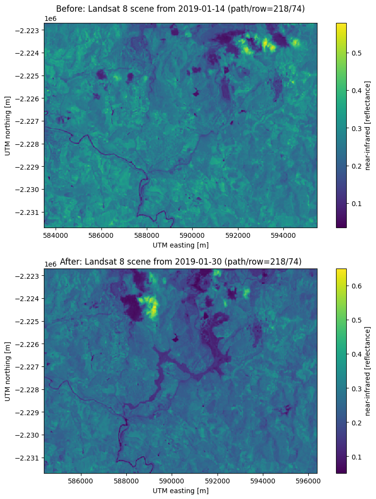
Plot some reflectance bands#
Now we can use the xarray.DataArray.plot method to make plots of
individual bands with matplotlib. A bonus is that xarray uses the
metadata that xlandsat.load_scene inserts into the scene to
automatically add labels and annotations to the plot.
import matplotlib.pyplot as plt

fig, (ax1, ax2) = plt.subplots(2, 1, figsize=(10, 12))

# Make the pseudocolor plots of the near infrared band
before.nir.plot(ax=ax1)
after.nir.plot(ax=ax2)

# Set the title using metadata from each scene
ax1.set_title(f"Before: {before.attrs['title']}")
ax2.set_title(f"After: {after.attrs['title']}")

# Set the aspect to equal so that pixels are squares, not rectangles
ax1.set_aspect("equal")
ax2.set_aspect("equal")

plt.show()
What now?#
Learn more about what you can do with xlandsat and xarray:
By getting the data into an xarray.Dataset, xlandsat opens the door
for a huge range of operations. You now have access to everything that
xarray can do: interpolation, reduction, slicing, grouping, saving to
cloud-optimized formats, and much more. So go off and do something cool!