Overview#
Why use xlandsat?#
One of the main features of xlandsat is the ability to easily read scenes
downloaded from USGS EarthExplorer into
xarray.Dataset along with all of the available metadata, which is very
useful for processing and plotting multidimensional array data.
We offer a simple and easy-to-use tool for smaller scale analysis and
visualization, which we can do thanks to the power of xarray.
When reading the data from the TIF files files using other tools like
rioxarray, some of
the rich metadata can be missing since it’s not always present in the TIF files
themselves.
Things like conversion factors, units, data provenance, WRS path/row numbers,
etc.
We take care of fetching that information from the *_MTL.txt files provided
by EarthExplorer so that xarray can use it, for example when annotating plots.
On top of that, xlandsat also offers tools for generating composites, pansharpening, histogram equalization, and more!
See also
More powerful (and more complicated) tools exist if your use case is beyond what we can handle. For cloud-based data processing, see the Pangeo Project. For other satellites and more powerful features, use Satpy.
The library#
All functionality in xlandsat is available from the base namespace of the
xlandsat package. This means that you can access all of them with a
single import:
# xlandsat is usually imported as xls
import xlandsat as xls
Download a sample scene#
The xlandsat.datasets module includes functions for downloading some
sample scenes that we can use. These are cropped to smaller regions of interest
in order to save download time. But everything we do here with these sample
scenes is exactly the same as you would do with a full scene from
EarthExplorer.
As an example, lets download a .tar archive of a Landsat 9 scene of the
city of Manaus, in the Brazilian Amazon:
path_to_archive = xls.datasets.fetch_manaus()
print(path_to_archive)
/home/runner/.cache/xlandsat/main/LC09_L2SP_231062_20230723_20230802_02_T1-cropped.tar.gz
The fetch_manaus function downloads the data file
and returns the path to the archive on your machine as an str.
The rest of this tutorial can be executed with your own data by changing the
path_to_archive to point to your data file instead.
Tip
The path can also point to a folder with the .TIF and the *_MTL.txt
file instead of a .tar archive.
Note
Running the code above will only download the data once. We use Pooch to handle the downloads and it’s smart enough to check if the file already exists on your computer.
See also
If you want to use the full scenes instead of the cropped version,
use pooch.retrieve to fetch them from the figshare archive
https://doi.org/10.6084/m9.figshare.24167235.v1.
Load the scene#
Now that we have the path to the tar archive of the scene, we can use
xlandsat.load_scene to read the bands and metadata directly from the
archive:
scene = xls.load_scene(path_to_archive)
scene
<xarray.Dataset> Size: 5MB
Dimensions:   (easting: 851, northing: 468)
Coordinates:
  * easting   (easting) float64 7kB 8.325e+05 8.325e+05 ... 8.58e+05 8.58e+05
  * northing  (northing) float64 4kB -3.55e+05 -3.55e+05 ... -3.41e+05 -3.41e+05
Data variables:
    blue      (northing, easting) float16 797kB 0.05908 0.05896 ... 0.06665
    green     (northing, easting) float16 797kB 0.07446 0.0752 ... 0.09082
    red       (northing, easting) float16 797kB 0.06152 0.06201 ... 0.1046
    nir       (northing, easting) float16 797kB 0.2915 0.293 ... 0.06409 0.06445
    swir1     (northing, easting) float16 797kB 0.1411 0.1434 ... 0.0509 0.05042
    swir2     (northing, easting) float16 797kB 0.07996 0.08093 ... 0.04968
Attributes: (12/19)
    Conventions:                CF-1.8
    title:                      Landsat 9 scene from 2023-07-23 (path/row=231...
    digital_object_identifier:  https://doi.org/10.5066/P9OGBGM6
    origin:                     Image courtesy of the U.S. Geological Survey
    landsat_product_id:         LC09_L2SP_231062_20230723_20230802_02_T1
    processing_level:           L2SP
    ...                         ...
    ellipsoid:                  WGS84
    date_acquired:              2023-07-23
    scene_center_time:          14:12:31.2799050Z
    wrs_path:                   231
    wrs_row:                    62
mtl_file: GROUP = LANDSAT_METADATA_FILE\n GROUP = PROD...Tip
Placing the scene variable at the end of a code cell in a Jupyter
notebook will display a nice preview of the data. This is very useful for
looking up metadata and seeing which bands were loaded.
The scene is an xarray.Dataset. It contains general metadata for the
scene and all of the bands available in the archive as
xarray.DataArray.
The bands each have their own set of metadata as well and can be accessed by
name:
scene.nir
<xarray.DataArray 'nir' (northing: 468, easting: 851)> Size: 797kB
array([[0.2915 , 0.293  , 0.2954 , ..., 0.2905 , 0.2905 , 0.2852 ],
       [0.2744 , 0.2788 , 0.2876 , ..., 0.2905 , 0.2837 , 0.2866 ],
       [0.2793 , 0.2769 , 0.2632 , ..., 0.3145 , 0.3247 , 0.3306 ],
       ...,
       [0.1864 , 0.1781 , 0.1835 , ..., 0.063  , 0.0641 , 0.06494],
       [0.1761 , 0.1761 , 0.2042 , ..., 0.06323, 0.0635 , 0.0642 ],
       [0.1791 , 0.1818 , 0.2052 , ..., 0.0646 , 0.0641 , 0.06445]],
      shape=(468, 851), dtype=float16)
Coordinates:
* northing (northing) float64 4kB -3.55e+05 -3.55e+05 ... -3.41e+05 -3.41e+05
* easting (easting) float64 7kB 8.325e+05 8.325e+05 ... 8.58e+05 8.58e+05
Attributes:
long_name: near-infrared
units: reflectance
number: 5
filename: LC09_L2SP_231062_20230723_20230802_02_T1_SR_B5.TIF
scaling_mult: 2e-05
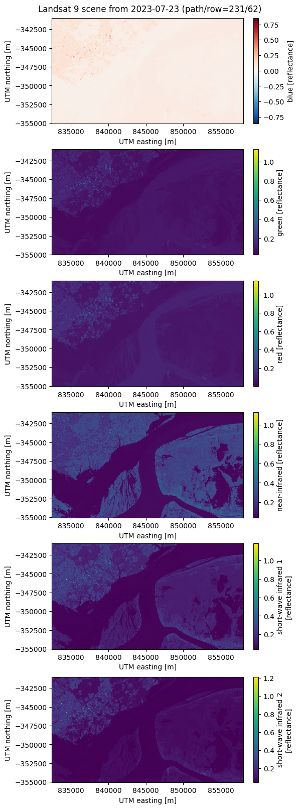
scaling_add: -0.1Plot some reflectance bands#
Now we can use the xarray.DataArray.plot method to make plots of
individual bands with matplotlib. A bonus is that xarray uses the
metadata that xlandsat.load_scene inserts into the scene to
automatically add labels and annotations to the plot:
import matplotlib.pyplot as plt

band_names = list(scene.data_vars.keys())

fig, axes = plt.subplots(
    len(band_names), 1, figsize=(8, 16), layout="compressed",
)

# Set the title using metadata from each scene
fig.suptitle(scene.attrs["title"])

for band, ax in zip(band_names, axes.ravel()):
    # Make a pseudocolor plot of the band
    scene[band].plot(ax=ax)
    # Set the aspect to equal so that pixels are squares, not rectangles
    ax.set_aspect("equal")

plt.show()
What now?#
Checkout some of the other things that you can do with xlandsat:
Plus, by getting the data into an xarray.Dataset, xlandsat opens the
door for a huge range of operations. You now have access to everything that
xarray can do: reduction, slicing, grouping, saving to cloud-optimized
formats, and much more. So go off and do something cool!